Japan’s demographic dilemma offers an opportunity for private equity
Scott Reynolds—Country Executive, Japan at Alter Domus—explores the implications of an aging population for investors in a recent article for Private Equity International
Scott Reynolds
Country Executive Japan
The piece examines the country’s evolving needs and challenges across sectors such as recruitment and healthcare, and the unconventional investment opportunities this shift creates. Scott highlights that the Japanese government is now taking steps to boost the population by encouraging immigration—up almost 44% since 2015.
What could this increase make possible for Japan’s economy—and how can investors benefit?
The Japanese government has historically been reluctant to open those gates, but this is slowly changing.
Alan Dundon, Director, Sales & Relationship Management at Alter Domus, and President of the Luxembourg Alternative Administrators Association (“L3A”), examines the outlook for private equity growth
Alan Dundon
Director, Sales & Relationship Management
Alan identifies three key drivers that are opening up new opportunities for investment managers, from the continuing democratization of alternatives to a growing focus on ESG. He also examines why Luxembourg’s alternatives community is still ambitious and why the jurisdiction continues to hold significant attractions for investment managers.
Investment managers looking to raise capital in Europe have traditionally looked and will continue to look to Luxembourg to establish their fund and operating platforms.
Alan Dundon, Director, Sales & Relationship Management
Demand for private credit allows lenders to regain control
Paolo Malaguti, Head of Credit-Vision, Alter Domus’ credit portfolio monitoring platform, discussed the outlook for private debt managers with IPE Magazine
Paolo Malaguti
Head of Credit-Vision
After a difficult period over the last 12 months, the latest forecasts from Preqin suggest that the private debt market is once again picking up pace and is set to reach global AUM of $2.53trn by 2027.
The supply and demand dynamics in private debt have changed: after several years of borrowers being able to negotiate what could be seen as overly-favorable conditions, the tide is turning towards the lender. Capital is available, but lenders are now able to demand more stringent covenant packages and higher yields.
Paolo dives into what this means for the asset class in terms of risk-return and how can new and how established managers can ensure they take full advantage of the opportunities.
This article was originally published in IPE Magazine.
Alter Domus supports Longship Fund III close at NOK2.1bn
Alter Domus (Guernsey) Limited is delighted to have supported Longship AS, a Norwegian-based private equity investor with a focus on the Norwegian lower-mid market, with the first and final closing of Longship Fund III.
Alter Domus
Following a successful migration of the fund administration role on Longship Fund I and Longship Fund II to Alter Domus in 2022, our Guernsey fund services team has been working closely with Longship and its advisers to deliver this closing.
With commitments raised of NOK2.1bn, Longship achieved the hard cap for their third fund in less than four months, with strong demand from institutional investors, including a 100% re-up rate from existing Longship investors.
In selecting Alter Domus in 2022, Longship were promised both a smooth migration process and an efficient set-up of new funds. Alter Domus have delivered on both.
Erik Rian Johannessen, CFO at Longship
The Alter Domus team comprised Tom Amy (Country Executive), Jordan Smith and Sarah Lacey (Senior Managers) and Raitis Darags (Manager).
We are thrilled to have the opportunity to now work with Longship across their three active funds. Using technology effectively, our fund services professionals have a depth of experience in supporting client migrations and delivering consistent, high standards of ongoing administration services.
Tom Amy, Country Executive Guernsey at Alter Domus
How rapid prototyping can kickstart companies’ digital transformation
How prototyping fintech products can develop business agility, change customer perception, and generate value faster
Curt Beck
Data Intake Analyst
Sandy McCarron
Head of Program Management and Team Operations
Teams talk about digital transformation, but many struggle to embrace it. It can be costly, time consuming, and the sheer amount of legacy technology that needs addressing can be overwhelming. Yet digital transformation doesn’t always require a large time or financial investment to start. At Alter Domus, we’ve established a transformation playbook to effectively jumpstart our digital transformation journey, building and revamping systems and applications rapidly, while being methodical- and most critically – customer focused.
A technique employed at Alter Domus is Rapid prototyping – an approach that allows teams to test a product idea quickly and inexpensively with clients to gain early insights into their pain points and how to solution them. There are multiple ways to prototype depending on need and time available – a throwaway prototype made in a couple hours to a full five-day Design Sprint, requiring a team to clear calendars, roll up their sleeves and make decisions together quickly.
Case study: Document tracker to DealFact
As data in the alternatives marketplace compounds and outgrows the spreadsheet, the Data & Analytics team saw an opportunity for a SaaS application that stores and manages all documents specified in a credit agreement between a borrower and lender.
Lenders are required to receive and keep track of important financial information from their borrowers, and that process was typically being performed via email and local spreadsheets, a manual process that required multiple follow ups and chasing, as there was no one place where all the documents were stored, making it very challenging for the lender to determine if they were receiving all the documentation outlined in the credit agreement.
The team started quickly building a prototype leveraging an existing internal tool that allowed users to upload and store all their documents in one place, giving them a clear picture of what’s been submitted and what was missing. We then met with domain experts from other areas within Alter Domus that managed Credit Agreements on behalf of clients to understand that workflow and the requirements needed.
It was crucial that the initial set of requirements reflected only the core functionality, enabling the developers to move with speed while at the same time putting a compelling solution in front of our clients. After two weeks of prototyping, the initial app was previewed to product strategy, members of the sales team, and select prospects to elicit feedback. The key was the development team was given maximum space to build the initial app before fully deciding functionality, and that the process was iterative, enabling the development to continuously move with velocity.
One of the more critical activities during this phase was partnering with the Commercial team to ensure that the prototype told a story that aligned with their view of what the market needs and resonated with prospects. We quickly validated the idea and affirmed the potential market need opportunity at hand, so the team moved to a full Design Sprint to dive deeper into the client needs and build out a more polished interactive prototype to share with existing clients.
Google Ventures notably developed the Design Sprint process to help clients validate their product hypothesis before investing in the actual product build. This approach also condenses the time-consuming efforts of understanding requirements and getting customer feedback on a realistic prototype – commonly a 3-6 month process – into one week.
Here’s an overview:
Monday: Map
Structured conversations allow the team to understand as much information on the concept as quickly as possible, defining key questions and a long-term goal. The sprint teams make a simple map of the product or service, speak to experts and ultimately pick a target.
Tuesday: Sketch
The team sketches ideas about how to best solve the market need (i.e., the problem that needs to be solved), focusing on individual thinking over a group brainstorm. Participants sketch their own detailed, opinionated solutions, emphasizing critical thinking over artistry.
Wednesday: Decide
The Facilitator leads the team through a gallery walk of Tuesday’s sketches and the team decides which should be prototyped and tested with clients by using silent votes over discussion to identify the best solutions. One “decider” picks the best of the best solutions which are combined into step-by-step storyboard for the prototype.
Thursday: Prototype
The Designer builds a realistic prototype of the storyboard that simulates a finished product for customers to get the best possible data from test, and you’ll learn whether you’re on the right track.
Friday: Test
The team shares the realistic prototype with five customers in five 1:1 interviews. The Facilitator asks targeted questions in a way to elicit unbiased feedback to the team’s most pressing questions.
At the conclusion of the sprint, customer feedback would dictate if the idea is viable or not. Some teams find out after a sprint that the idea doesn’t have an audience. For us it was clear that our prototype resonated with interviewees, giving us the go-ahead to transition from high fidelity prototype to building an MVP Product.
The requirements and ideas gathered during prototyping became the basis for a product backlog. Following Agile Development methodology, our product, design, and development teams prioritized this backlog and built a validated idea into a shippable product in roughly seven months. DealFact is currently available for clients.
Highlights
The Quant team built an application that tracked Loan Trade Settlement times, giving the Loan Trade Settlement team and their clients key insights into how to more effectively manage trade settlement.
In a week, our Quant team built a dashboard that highlighted our financial spreading capabilities.
The Credit Vision team used a Design Sprint to gain alignment on critical new features and reimagine the user experience for its next generation relaunch (pending Q3 launch).
Recognizing the need for a centralized portal for our client-facing products, a Design Sprint was held in January for AD Storefront, to broaden our clients’ awareness of all our products and services, and act as the single “front door” for our clients to log into their respective products (pending Q2 launch).
Alter Domus wins ‘Best Fund Administrator – Private Debt’
The Private Equity Wire European Awards ceremony took place on March 8th in London
Alter Domus
We’re delighted to have been named ‘Best Fund Administrator – Private Debt’ at the Private Equity Wire European Awards 2023 in London. Following on from our win in the same category at the US awards in November 2022, this coveted award is testament to the growing breadth and depth of our expertise in the field around the globe.
The award recognizes the exceptional growth and development of our Private Debt Solutions across Europe, reflecting our team’s ability to provide market-leading support for private debt managers, meeting their operational, data and transparency requirements. We are particularly proud that the award is voted for by our industry peers.
Patrick McCullagh, Juliana Ritchie, Lora Peloquin and Matthew Molton attended the awards ceremony at The Reform Club in London on 8 March to accept the award and to celebrate the achievement with partners from across the industry.
We are delighted to win this prestigious award this year, which reflects the quality of our service offering and our reputation within the private debt market. Alter Domus continues to grow its private debt services globally, providing true end-to-end solutions to our clients.
Juliana Ritchie, Head of Sales & Relationship Management, Debt Capital Markets, Europe
Presenting a fresh perspective on assessing credit losses of CLO portfolios
Rudolph Bunja
Head of Portfolio Credit Risk
As structured finance market participants are aware, notes issued by collateralized loan obligations (CLOs) introduce varying credit exposures to the underlying corporate leverage loan portfolio based on the relevant notes’ cashflow priority. This therefore offers investors the opportunity to participate in this asset class based on their own risk and cash flow preferences.
An assessment of how the underlying risk is distributed across the notes is fundamental for investors and other market participants. Obviously where that risk comes to bare and CLO credit losses are incurred, there are challenges to estimate and allocating that loss. To explore this complex issue and to come to an understanding of the outcome of credit loss, we ask two fundamental questions:
Firstly, how is the total portfolio credit loss allocated across the CLO’s notes? And, secondly, what is the total loss of the underlying portfolio that is to be allocated to the CLO’s notes?
Based on our analysis, we find that:
The first loss equity tranche absorbs most of the estimated portfolio credit losses.
Estimating portfolio credit losses is as much an art as a science and is subject to significant judgment.
Excess interest and other structural deal features could materially reduce the estimated portfolio credit loss and the allocation of such losses across the CLO’s notes – translation: the answers to the questions above could vary substantially once excess interest and structural deal features are considered.
A Simple Example to Demonstrate CLO Complexities
In order to illustrate both the complexities of estimating portfolio credit losses and how the estimated loss distribution of an underlying pool of leveraged loans may be allocated across a CLO’s capital structure, we have created a simple example. To begin, we assume a static portfolio of loans that is well diversified, with certain homogeneous characteristics (e.g., credit quality, maturity, seniority) and has a total par amount equal to the amount of CLO notes issued.
Furthermore, we assume the CLO has a simple capital structure with three classes of notes (Class A, B, and equity) paid in order of straight sequential seniority. For simplicity, we ignore interest payments and discounted cashflows. We assume no interest on the collateral, nor on the CLO’s tranches.
This assumption is an important building block to gain a good understanding of how losses are measured and allocated to the CLO’s tranches. These assumptions will ensure that the total credit loss of the portfolio will equal the aggregate credit losses allocated to the CLO’s tranches.
Relaxing these assumptions, which may be considered for possible future research, is relevant since excess interest is typically available to a CLO where the cash flow priority rules serve first to reduce the amount of portfolio credit loss that is allocated to the notes and secondly reorder the allocation of the remaining losses.
Thus, to a certain extent, our simplified CLO is a ‘worst case scenario’ for the notes. In our stylized example, the only credit enhancement for the CLO’s notes is through overcollateralization (OC) based on the par amount of the underlying loans, similar in structure to a CLO overcollateralization test. In this case, the total amount of principal that can be distributed across the tranches is equal to those received on the loans. By extension, the total credit losses of the underlying portfolio are equal to the credit losses that are allocated to the CLO’s tranches in our simplified case.
Equation #1: Losses Allocated to the CLO Tranches = Total Portfolio Credit Loss
Importantly, as you read on, we’ll introduce an extended equation that represents the true nature of CLOs by incorporating excess interest.
How are Portfolio Credit Losses Allocated?
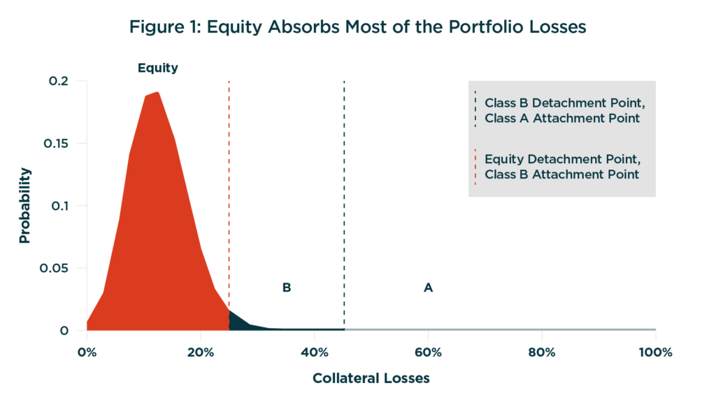
Figure 1 displays a hypothetical portfolio loss distribution where the thresholds along the x-axis indicate the relevant notes’ amount of credit enhancement based on the capital structure. Each notes’ probability of loss and EL are indicated by the curve exceeding its amount of credit enhancement and the cumulative probability within each notes’ thresholds, respectively. The maximum amount of loss is equal to the total amount of notes.
As to be expected, the more senior the note, the lower the likelihood of loss which is indicated by the ‘tail’, whereas the equity absorbs most of the CLO portfolio’s EL as we see in Figure 1. In actuality, the equity absorbs over 95% of the total loss in this example. Note also that the ELs across the notes is equal to the EL of the underlying pool. So, here’s our first insight:
Equity tranche absorbs the vast majority of portfolio losses
How are Portfolio Credit Losses Estimated?
The weighted average probability of default (‘PD’) and loss given defaults, which are represented by the credit quality of the pool, define the mean of Figure 1, while the shape of Figure 1 is based on various diversification elements (e.g., issuer/sector exposure). Estimation of these variables is not an easy task.
For example, what PD should be used to map to a credit quality of a borrower? Also, what duration should be assumed (e.g., stated maturity or expected life) as historical default rates indicate that default rates and credit losses increase with time horizons. This leads us to the second challenge in performing this analysis – namely, what is the assumed credit loss of the underlying CLO?
To a casual reader, the expected credit loss of the underlying portfolio may simply be the product of the average PD of the underlying collateral multiplied by the average loss rate. But let’s be a bit more precise by referencing historical credit loss observations[1].
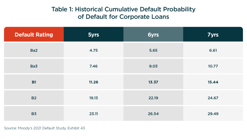
Table 1 below shows cumulative default rates for corporate debt over a 5-year, 6-year and 7-year horizon for select speculative grade ratings. We have highlighted the B1 row, as an example, assuming our stylized CLO consists of B1-rated corporate issuers.
Using a 7-year weighted average life (‘WAL’) and a B1 rating the expected default rate is roughly 15.44%. Assuming an average recovery of 50%, this would translate into an expected loss rate of 7.72% (15.44% * 50% loss rate). Note that recovery rates are also subject to change depending on market conditions. For simplicity, in this paper we assume that recovery rates are fixed at 50%.
Historically, a 50% recovery rate for a first lien senior secured loan is a conservative estimate – especially since in our stylized example we assume that the portfolio loans are rated one rating sub-category higher than the PD rating. However, the assumption of which WAL and which PD to use is not that simple.
Why not use the actual WAL and actual WARF?
CLOs are subject to a WAL test. Practically speaking, CLO managers endeavor to actively manage the portfolio such that there is a cushion between the portfolio’s actual WAL and the test level. Like the WAL test, CLOs typically have an average credit quality test (Weighted Average Rating Factor or ‘WARF’).
In this example, we can assume the test has been set to the B1 rating level. CLO managers will also endeavor to manage their portfolio to maintain a cushion between the actual WARF and the test level. As a result, CLOs will typically be managed to have true PDs that are lower than those indicated by their test levels.
Further reducing the WAL of a CLO portfolio are underlying corporate loan prepayments – both scheduled and unscheduled. Prepayments would further reduce the WAL of the portfolio, which by extension reduces PD and credit losses.
Which combination of WARF, WAL, and WAS to use?
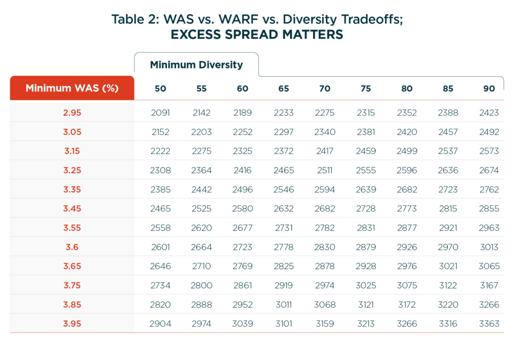
CLOs typically allow managers the flexibility to offset collateral quality test cushions. The WARF tests, for example, will often vary based on the Weighted Average Spread (‘WAS’) and other portfolio characteristics. These tradeoff opportunities are often documented in a dynamic matrix within the CLO.
Excess spread is often a critical component of the CLO. These tradeoff options, illustrated in Table 2[2] below, give us some hints about the reduction in the EL of the portfolio after considering the effects of excess spread, or WAS.
For example, assume a CLO with a given diversity of 50, the WARF could be as low as 2091 (with a WAS of 2.95%) and as high as 2904 (with a WAS of 3.95%). The difference translates into a one third reduction in the portfolio’s WARF and EL due to excess interest of 100bps – excess interest matters!
This example highlights the importance of excess spread in estimating ELs for the CLO’s notes. Excess interest reduces the amount of CLO portfolio losses that are allocated to the notes – a topic for possible future research. Which leaves us with the following further insights:
Estimating CLO portfolio principal credit losses is very difficult to assess and could change dynamically.
Excess interest reduces the total losses to the CLO’s tranches – i.e., total losses allocated to the tranches is less than the total portfolio credit losses.
The last insight allows us to update Equation #1 with Equation #2 below, which is more accurate in estimating net portfolio losses that are to be absorbed by the CLO’s notes.
Equation #2: Losses Allocated to CLO Tranches = Total Portfolio Credit Losses – Excess Interest
Items for considerations
In contrast to the above stylized example where we demonstrated some of the fundamental challenges in measuring credit losses, CLOs are more complex. They include intricate cashflow waterfalls that segregate interest and principal collections, which incorporate key structural features (e.g., OC tests) within the cashflow waterfall that can have implications for the notes.
An assessment of these features, which is beyond the scope of this paper, would be part of a more comprehensive analysis of portfolio losses and allocation of those losses to CLO notes. We would expect that these features to reduce the CLO’s portfolio losses and to skew the allocation of the reduced losses to favor the more senior notes.
In Conclusion
Estimating credit losses for a CLO portfolio is not an easy task. Various assumptions need to be made, including the appropriate WAL and PD (or WARF). With simple and reasonable assumptions, we’ve shown that estimated portfolio loss rates could vary significantly. Allocation of losses across the tranches adds another layer of complexity though we showed that the equity tranche will bear the brunt of the portfolio losses – over 95% in our stylized CLO.
CLOs incorporate features that could further reduce the underlying portfolio losses and change the allocation of those losses. We described how excess interest reduces portfolio credit losses that are allocated to the tranches, and that structural features such as OC tests can reduce the amount of the loss that is allocated to the non-equity tranches. In summary, we conclude that:
The first loss equity tranche absorbs most of the estimated portfolio credit losses.
Estimating portfolio credit losses is as much an art as a science and is subject to significant judgment.
Excess interest and other structural deal features could materially reduce the estimated portfolio credit loss and the allocation of such losses across the CLO’s tranches.
US private debt market’s remediation plans will aid the successful transition away from LIBOR
Jason Mendoza
Senior Quant Modeler
Time, as they say, moves on relentlessly, and for financial institutions the clock is well and truly ticking down on the transition away from the LIBOR. Indeed, borrowers and lenders are acutely aware that in just months the long-utilized rate will cease to exist.
The need to successfully shift to an alternative rate such as the Secured Overnight Financing Rate (SOFR) is vital. LIBOR is the basis on trillions of dollars of loans and is tied to a multitude of products, such as adjustable-rate mortgages, student loans and corporate loans. Careful transitioning is the key to minimizing large-scale financial impacts, especially in the private debt market[1].
Now, as the deadline looms, it’s essential that we examine the two fundamental questions: what’s the current status of LIBOR transition in the U.S private debt space, and how well prepared are institutions for an orderly transition to the aforementioned new rates?
The impetus for change: LIBOR and the financial crisis
As the dust finally began to settle on the financial crisis, public scrutiny in mid-2012 turned sharply to focus on LIBOR, which had been the standard reference rate for most adjustable-rate products for decades. The market was awash with allegations that during the financial turmoil, banks were misreporting borrowing rates in order to convey financial stability.
Since LIBOR was calculated from self-reported bank submissions, banks could in theory change the submissions and influence the published LIBOR value. In the wake of the allegations, financial regulators around the world urged financial institutions to move away from LIBOR. In 2014, the Alternative Reference Rates Committee (AARC) was created by the Federal Reserve Board and the New York Fed to support the transition away from LIBOR.
In 2017, the AARC then recommended the SOFR, a measure of the cost of borrowing overnight collateralized by Treasury securities[2], as the preferred alternative rate. This is primarily because SOFR is thought to be less susceptible to manipulation and is based on a vast volume of daily transactions (nearly $1 trillion), as opposed to LIBOR (estimated $500 million).
The early struggle to adopt SOFR
While it was helpful to determine an alternative rate, market participants struggled to quickly adopt SOFR, for various reasons. First, SOFR is a risk-free rate since it is backed by the U.S treasury. The LIBOR rate, however, incorporates credit risk (between banks) in the rates, and therefore tends to be higher. If lenders are to adopt SOFR, they need to add this incremental credit risk. To address this issue, the AARC also provided guidance on an additional “credit adjustment spread” to add to the SOFR rate when transitioning away from LIBOR[3].
Moreover, SOFR is an overnight rate, whereas LIBOR contains various terms/tenors (overnight, 1-week, 1 month, 2 month, 3 month, 6 months and 12 months). To address this gap, the AARC suggested the CME Term SOFR in July 2021, which modifies SOFR to have the same terms/tenors as LIBOR[4].
Timeline of transition
Now that lenders/borrowers are equipped with alternative rates that are most consistent with LIBOR, what are the key dates they should have in mind regarding the transition? The 1-week and 2-month LIBOR rates were discontinued in Dec 31, 2021, and loan originations after that date should for the most part be pegged to an alternative rate[7]. The most important deadline is June 30, 2023, which is when all LIBOR rates would irrevocably be discontinued, and every LIBOR rate loan should be moved to an alternative rate.
The state of play: Where do US private debt markets stand?
Bank loan originations tied to SOFR in 20222: On track
New bank loan originations in 2022, which post Dec 31, 2021, should not be pegged to LIBOR, went according to expectations. Based on data from Refinitiv, a large majority of syndicated US loans originated in 2022 were priced to Term SOFR. For the non-regulated direct lending market, however, the share of new originations priced to Term SOFR was closer to 50%[8].
The transition to SOFR was generally smoother than what lenders were expecting, largely in part to AARC’s recommendation of the CME Term SOFR back in July 2021[9], which helped generate a term structure akin to LIBOR.
Transitioning remaining loans to SOFR: long road ahead but room for optimism
So what about the remainder of loans, originated prior to 2022, that still need to transition away from LIBOR? According to the LSTA[10], using data from LevFin Insights, the CS Loan Index, Refinitiv LPC and CLO surveillance reports, roughly 15% of broadly syndicated loans are currently on SOFR. What about the direct lending space? As a proxy, we turned to publicly available BDC data. From a sample of 12 BDC’s (Business Development Companies) registered with the SEC, all but three BDCs had between 12% to 30% of their books currently pegged to SOFR. In this sample, the average transition rate was 15%, exactly what is estimated for the broadly syndicated loan market. The general 15% LIBOR transition rate may seem small, considering how near LIBOR cessation is, but to further understand that number we can turn to the Loan Remediation Survey[11][12], recently administered by the ARRC. The survey ran from August 9 to through September 7, 2022 and is comprised of 73 submissions; lenders and borrowers comprise of roughly 70% and 30% of the responses, respectively. Across all respondents, 89% had a loan remediation plan, which suggests that, even though there doesn’t appear to be much activity, there is significant planning that is yet to manifest. Across all agents or bilateral lenders, 94% have identified all LIBOR loan exposures, 75% have contacted borrowers regarding their remediation plans and 75% have begun to actively transition loans away from LIBOR.
How do lenders and borrowers intent to transition the remaining loans?
It is encouraging to see that there is considerable planning and action taking place to transition away from LIBOR, but what methods are most adopted? 64% agents or bilateral lenders began to remediate contracts by adding “hardwired” fallback language. From the borrowers that were contacted, however, only 13% were receptive to amending “hardwired” fallbacks and 4% wanted to rely on existing fallbacks at cessation.
The most popular response, by 46% of borrowers, was to refinance directly to the replacement rate. In this environment of high inflation and economic uncertainty, getting favorable terms in a refinance may be challenging and could cause a backlog without a backup plan, like an amendment.
What timeline do lenders and borrowers have in mind?
With regards to timing, 86% of agents/lenders expect most of their loans to transition away from LIBOR by the end of 2023Q2, or the last available quarter where LIBOR will be published. At 43%, half the agents/lenders expect to transition in 2023Q1 or earlier, leaving a potential backlog come 2023Q2. The remaining 14% of agents/lenders expect most loans to be transitioned after 2023Q2, which may seem concerning.
However, from those 14%, 70% of lenders report that a vast majority of their loans have hardwired fallback language, which means that loans would automatically revert to an alternative rate at LIBOR cessation.
Alter Domus’ role in the LIBOR transition
As a leading agent in the private debt markets, Alter Domus has proactively reached out to our clients to make sure they were preparing for the transition of their portfolios. Using our recommendations and reporting tools, our clients are prepared for the end of LIBOR in 2023.
The Reasons for Market Optimism
Although the percentage of loans currently transitioned away from LIBOR in the private debt space, 15%, seems rather small, there is reason to be optimistic. Thanks to the Loan Remediation Survey, there is data to support considerable LIBOR remediation plans by 89% of market participants. While the loans might not be transitioned currently, most loans have either AARC hardwired fallbacks (where transition is triggered automatically after LIBOR cessation) or amendment fallbacks, which would mean an amendment would have to be raised.
If action is taken early enough, the private debt market can avoid a costly and risky backlog of amendments. With the end of LIBOR coming within the next six months, we will continue to provide timely updates as warranted, in line with evolving private debt trends.
Risk-Managing Trade Settlement in Alternative Debt Markets
Steve Kernytsky
Manager, Quantitative Analytics
The favorable risk-return characteristics of private debt are attributed to a variety of factors, including compensation to sophisticated investors for accepting limited liquidity and increased complexity relative to the liquid public markets. A contributing factor to the liquidity premium in the private debt market is the cost and related risk of trade settlement.
Trade settlement in the private debt market is a complex process and is often subject to the unique characteristics of the traded facility. At times, trades could take months to settle, exposing buyers and sellers alike to significant risks around volatility, losses and cash flow management. However, there are certain factors that could assist private debt investors to better assess and manage the risks associated with trade settlement.
Loan Trade Settlement – Not a Transitory Consideration
At Alter Domus, our Loan Trade Settlement group continues to see significant growth in trading volumes, well in excess of the LSTA volumes, as we continue to maximize efficiency, flexibility, and reliability for our clients. With the anticipated continuing growth of the private debt markets, we expect trading volumes to maintain their current upward trajectories, further highlighting the importance for investors to better understand and manage the risks associated with loan trade settlement.
Why Should I Care?
Trade settlement exposes buyers and sellers to several risks. Trades could take a relatively long period of time to settle. These longer time periods pose challenges to buyers and sellers to forecast and manage their cash flows – an important consideration for fund managers looking to satisfy, for example, (i) investor redemptions (seller), (ii) commitments to purchase other loans (seller), or (iii) investment objectives (seller and buyer). Delayed settlement could also pose significant incremental administrative challenges and costs to trade counterparties. In a nutshell, delayed and unpredictable trade settlement imposes costs and operational challenges and risks to the front, middle and back offices of sophisticated alternative debt investors.
As already noted, one of the most notable traits of loan trade settlement is the wide variation in times to settle. While public equity and bond traders can confidently expect that the trades initiated on a given day will close in a narrow and predictable time span, private loan traders have no such luxury.
Consider a secondary, non-distressed loan on the LSTA market, the most common loan type traded. A well-behaving trade might close in a little under 20 business days. But things don’t always go so smoothly. Sometimes the process is initiated, but then stalls immediately. Sometimes the process is near completion, only to have the agent point out that the key parts of the signoff are still pending, such as KYC or Borrowers’ Consent. Sometimes these challenges occur as the quarter is nearing its conclusion and the Agent puts all transfers on hold for several days due to scheduled principal or interest activity. At this point, the still open trade is now at 45 days, and may not close for another week or more as the factors contributing to the delay are resolved. As such, even in the secondary LSTA market, loan settlements in the 60-90 days range are not rare.
During a prolonged settlement period, risks could emerge – for example, market conditions could shift, interest rates could change beyond expectations, or the borrower’s risk profile could change.
Similarly, loan managers face additional challenges regarding cashflow management. Anytime a given loan trade settles, cash reserves are affected. Loans committed to be purchased or fund investor redemptions require cash to complete the transaction. Loans sold will lead to an inflow of cash that could be used to meet those commitments. As alternative debt managers continue to gain better insights into the timing of loan settlement, they could further improve their overall fund operations.
Given these potential challenges, it is no surprise that traders would want to factor time to settlement risk into their decision-making process. The good news is that there are several factors that could assist traders to better quantify and manage their trade settlement process. Importantly, while in this paper we share generic observations about the loan trade settlement process, each alternative debt investor will often face unique risks given their portfolio strategy. At Alter Domus, our Loan Trade Settlement team considers these factors and works closely with our clients to provide greater transparency into their unique risks.
What are the Indicators of Loan Settlement Risk?
Loan Facility and Market Characteristics
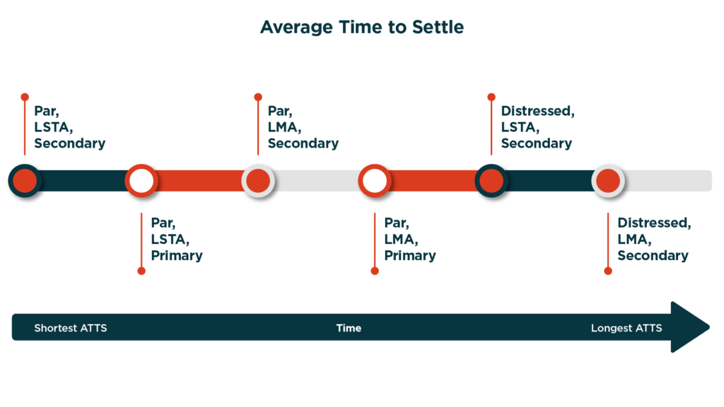
The most visible factors impacting loan trade settlement are; (i) the trading market (LMA vs. LSTA), (ii) the borrower’s financial condition (‘Par’ loans for financially healthy borrowers and ‘Distressed’ loans for financially stressed borrowers), and (iii) whether the trade is a primary versus secondary market trade. Par LSTA loans are the fastest loan type to close, typically closing in under 25 business days. Par LMA loans take somewhat longer, coming in just under 60 days across both markets. In both the LSTA and LMA Markets, Secondary Par Loans close faster than Primary loans. On the other hand, Distressed loans across both LMA and LSTA are the longest to settle, with distressed LMA loans being the longer of the two.
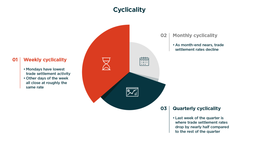
Cyclicality
Weekly, monthly, and quarterly cyclical elements come into play for determining loan settlement. At the weekly level, all else equal, Mondays often seem to have the lowest trade settlement activity, while the other days of the week close at roughly the same rate.
While at the weekly level the start of the week is where settlement slows the most, the monthly and quarterly patterns are the opposite. As month-end nears, settlement rates decline quite a bit. This pattern appears to be particularly strong, during the last week of the quarter.
Trade Activity for the Loan
The Loan Identifier can indirectly become a quite useful variable to better understand trade settlement risk. By tracking repeat loan trades using the loan identifiers, we have noticed that loans that have traded repeatedly tend to settle much faster than less frequently traded loans. Intuitively, this is not surprising. As a loan facility’s trading activity increases, the administrative process to settle trades improves as kinks in the settlement process are addressed and corrected through repeated activity.
Counterparties, Agents and Others in the Settlement Process Ecosystem
Intuitively, the counterparties and agents involved in a trade would affect how smoothly a given trade settlement process might go. Traders might have an awareness that certain counterparties or agents have been very effective in the past, or vice versa. The data supports such intuition. Counterparties and agents have historic patterns regarding their trade settlement effectiveness.
Conclusion
The factors that affect loan trade settlement times are very relevant for private loan traders. Implications include cash flow management challenges, potential losses, and costs related to delayed trades. These associated challenges are not transitory. The market continues to grow as investors expand their allocations to this appealing asset class.
We’ve identified several factors that could help traders better manage this risk. But we do caution that aggregated market data from industry sources can only tell part of the story. Each client will have their own unique trading profile, and only by exploring the nuanced specific data could traders more precisely quantify their unique risks. Alter Domus will continue to support the loan trade settlement marketplace in our ongoing mission to provide insights to our clients that helps them manage and quantify their trade settlement risk.